2D Quadrotor Optimization

Repository

Mathematica Code this file has .nb extendion and can probably only be read properlly with Wolfran Mathematica

The derivation of the control equations can be found here.

Introduction

As my final project for the Numerical Methods in Optimal Control class I applied a Gradient Descent and some of its different techniques (e.g. Armijo Theorem, Ricatti Theorem, trajectory projections) on quadrotors, one of my main areas of interest. The goal is to optimize the force input needed to be generated by its rotors in order to be compliant to a given trajectory in the best way possible according to its dynamics. For this project I used Wolfram Mathematica, the recommended software for the class and due to its facility in performing symbolic calculation, plots and animations. However, Mathematica does not achieve the same performance as languages such as C++ and since complex calculations will need to be done, one of the drawbacks of this project is the time it takes processing before generating an animation. In order to optimize the process by simplifying the math, I reduced the number of differential equations in the dynamics of the quadrotor, so let’s assume instead we are using a “dualrotor” the quadrotor of the 2D world, as shown in the scheme bellow:

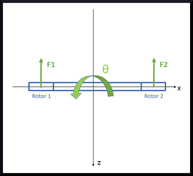
In the representation above the X-axis points to the righ, the Y-axis points to the interior of the screen and the Z-axis points down. F1 and F2 are forces caused by the trust generated by the rotors 1 and 2, which can move the “dualrotor” by translations in XZ-plane and a rotation ϴ around the Y-axis (Pitch).

Code and Animation

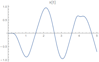
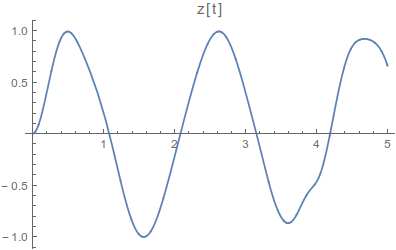
The algorithm will provide an animation of a bar like 2D Quad rotor as well as the plots for {x, z, ϴ}.

2DQuad_Loop from Guilherme Klink on Vimeo.

Getting a 2D-Quadrotor

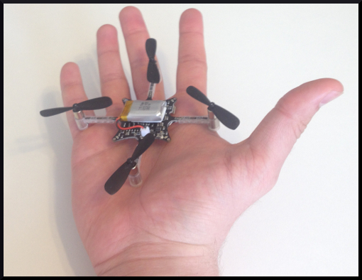
A quadrotor is a flying machine composed by four rotors equidistant from each other, with center of mass in its middle. Its flight is controlled by the difference of upward forces generated by the thrust of each rotor as schematized in the figure bellow.

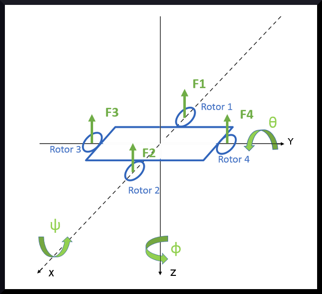
Disconsider 2 rotors

In a 2D representation we are going to assume that rotors 3 and 4 do not produce thrust (therefore F3=0 N and F4=0 N) and to eliminate Yaw (φ) we have to assume the propellers do not create any Hub horizontal force on its blades.

Move only in one plane

Since we are not considering rotors 3 and 4 we can eliminate Roll (ψ). The quad rotor cannot move without tilting for the direction it wants to go, therefore it needs to roll to be able to move on the Y-axis, thus since we eliminated roll, from now on it will only be able to move on the 2D plane XZ.

Remaining degrees of freedom

We end up with the following possible movements that will be used to compose the 2D Quad rotor state with 3 DOF:

• X: when the quad tilts with ϴ it can moves in the X-axis
• Z: the movement in this axis is defined by the sum of the z-components of F1 and F3.
• ϴ: it can tilt by the resultant moment of F1 and F2.

2D-Quadrotor dynamics

The derivation of the dynamics of the 2D-Quadrotor can be seen at Section 1 of the write up.

The Projection

For our gradient descent algorithm it is important to have a good Projection function (denoted by P). The projection function has the purpose of converting any simplified non-feasible state to a feasible state, in other words, it converts to a state that is compliant to the quadrotor dynamics. The way this function can be obtained is showed in Section 2.

The Cost Function

A basic quadratic cost equation was used since this types of functions generate a parabola. The reason a parabola cost function is interesting for a gradient descent algorithm is that for this particular shapes the local and global minimum coincide (as shown in the figure below).

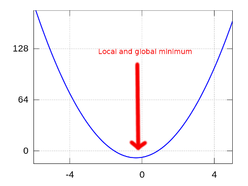
Therefore is guaranteed that the algorithm will always be able to find the lowest cost without getting stuck in a local minimum. The specific quadratic function used as the way its constants were tuned can be found in Section 3.

Armijo Line Search

The Armijo line search innequation is used to guarantee that on each step the gradient descent will descent and eventually achieve an optimal solution.

Conclusion

Unfortunattelly, the Mathematica running performance makes this alghorithm unfeasable for a real life quadrotor aplication (it would run for hours and problem overflow the computer’s memory), however it was important for my understanding of how implement a Gradient Descent Optimization for a complex problem and to polish my skills with quarotor dynamics. I hope in the future to implement the same solution using a faster programming language.